The Annotated Transformer
The recent Transformer architecture from “Attention is All You Need” @ NIPS 2017 has been instantly impactful as a new method for machine translation. It also offers a new general architecture for many NLP tasks. The paper itself is very clearly written, but the conventional wisdom has been that it is quite difficult to implement correctly.
In this post I present an “annotated” version of the paper in the form of a line-by-line implementation. (I have done some minor reordering and skipping from the original paper). This document itself is a working notebook, and should be a completely usable and efficient implementation in about 400 LoC. To follow along you will first need to install PyTorch and torchtext. The complete notebook is available on github or on Google Colab.
- Alexander Rush (@harvardnlp)
# !pip install http://download.pytorch.org/whl/cu80/torch-0.3.0.post4-cp36-cp36m-linux_x86_64.whl numpy matplotlib spacy torchtext # Standard PyTorch imports
import numpy as np
import torch
import torch.nn as nn
import torch.nn.functional as F
import math, copy
from torch.autograd import Variable
# For plots
%matplotlib inline
import matplotlib.pyplot as pltThe following text is verbatim from the paper itself. My comments are in the code itself. - AR
Background
The goal of reducing sequential computation also forms the foundation of the Extended Neural GPU, ByteNet and ConvS2S, all of which use convolutional neural networks as basic building block, computing hidden representations in parallel for all input and output positions. In these models, the number of operations required to relate signals from two arbitrary input or output positions grows in the distance between positions, linearly for ConvS2S and logarithmically for ByteNet. This makes it more difficult to learn dependencies between distant positions. In the Transformer this is reduced to a constant number of operations, albeit at the cost of reduced effective resolution due to averaging attention-weighted positions, an effect we counteract with Multi-Head Attention.
Self-attention, sometimes called intra-attention is an attention mechanism relating different positions of a single sequence in order to compute a representation of the sequence. Self-attention has been used successfully in a variety of tasks including reading comprehension, abstractive summarization, textual entailment and learning task-independent sentence representations. End- to-end memory networks are based on a recurrent attention mechanism instead of sequencealigned recurrence and have been shown to perform well on simple- language question answering and language modeling tasks.
To the best of our knowledge, however, the Transformer is the first transduction model relying entirely on self-attention to compute representations of its input and output without using sequence aligned RNNs or convolution.
Model Architecture
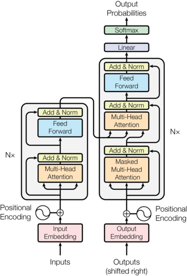
Most competitive neural sequence transduction models have an encoder-decoder structure (cite). Here, the encoder maps an input sequence of symbol representations $(x_1, …, x_n)$ to a sequence of continuous representations $\mathbf{z} = (z_1, …, z_n)$. Given $\mathbf{z}$, the decoder then generates an output sequence $(y_1,…,y_m)$ of symbols one element at a time. At each step the model is auto-regressive (cite), consuming the previously generated symbols as additional input when generating the next.
class EncoderDecoder(nn.Module):
    """
    A standard Encoder-Decoder architecture. Base for this and many
    other models.
    """
    def __init__(self, encoder, decoder, src_embed, tgt_embed, generator):
        super(EncoderDecoder, self).__init__()
        self.encoder = encoder
        self.decoder = decoder
        self.src_embed = src_embed
        self.tgt_embed = tgt_embed
        self.generator = generator

    def forward(self, src, tgt, src_mask, tgt_mask):
        "Take in and process masked src and target sequences."
        memory = self.encoder(self.src_embed(src), src_mask)
        output = self.decoder(self.tgt_embed(tgt), memory,
                              src_mask, tgt_mask)
        return output
The Transformer follows this overall architecture using stacked self-attention and point-wise, fully connected layers for both the encoder and decoder, shown in the left and right halves of Figure 1, respectively.
Encoder and Decoder Stacks
Encoder:
The encoder is composed of a stack of $N=6$ identical layers.
def clones(module, N):
    "Produce N identical layers."
    return nn.ModuleList([copy.deepcopy(module) for _ in range(N)])
class Encoder(nn.Module):
"Core encoder is a stack of N layers"
def __init__(self, layer, N):
super(Encoder, self).__init__()
self.layers = clones(layer, N)
self.norm = LayerNorm(layer.size)
def forward(self, x, mask):
"Pass the input (and mask) through each layer in turn."
for layer in self.layers:
x = layer(x, mask)
return self.norm(x)We employ a residual connection (cite) around each of the two sub-layers, followed by layer normalization (cite).
class LayerNorm(nn.Module):
    "Construct a layernorm module (See citation for details)."
    def __init__(self, features, eps=1e-6):
        super(LayerNorm, self).__init__()
        self.a_2 = nn.Parameter(torch.ones(features))
        self.b_2 = nn.Parameter(torch.zeros(features))
        self.eps = eps

    def forward(self, x):
        mean = x.mean(-1, keepdim=True)
        std = x.std(-1, keepdim=True)
        return self.a_2 * (x - mean) / (std + self.eps) + self.b_2
That is, the output of each sub-layer is $\mathrm{LayerNorm}(x + \mathrm{Sublayer}(x))$, where $\mathrm{Sublayer}(x)$ is the function implemented by the sub-layer itself. We apply dropout (cite) to the output of each sub-layer, before it is added to the sub-layer input and normalized.
To facilitate these residual connections, all sub-layers in the model, as well as the embedding layers, produce outputs of dimension $d_{\text{model}}=512$.
class SublayerConnection(nn.Module):
    """
    A residual connection followed by a layer norm.
    Note for code simplicity the norm is first as opposed to last.
    """
    def __init__(self, size, dropout):
        super(SublayerConnection, self).__init__()
        self.norm = LayerNorm(size)
        self.dropout = nn.Dropout(dropout)

    def forward(self, x, sublayer):
        "Apply residual connection to any sublayer with the same size."
        return x + self.dropout(sublayer(self.norm(x)))
Each layer has two sub-layers. The first is a multi-head self-attention mechanism, and the second is a simple, position-wise fully connected feed- forward network.
class EncoderLayer(nn.Module):
    "Encoder is made up of self-attn and feed forward (defined below)"
    def __init__(self, size, self_attn, feed_forward, dropout):
        super(EncoderLayer, self).__init__()
        self.self_attn = self_attn
        self.feed_forward = feed_forward
        self.sublayer = clones(SublayerConnection(size, dropout), 2)
        self.size = size

    def forward(self, x, mask):
        "Follow Figure 1 (left) for connections."
        x = self.sublayer[0](x, lambda x: self.self_attn(x, x, x, mask))
        return self.sublayer[1](x, self.feed_forward)
Decoder:
The decoder is also composed of a stack of $N=6$ identical layers.
class Decoder(nn.Module):
    "Generic N layer decoder with masking."
    def __init__(self, layer, N):
        super(Decoder, self).__init__()
        self.layers = clones(layer, N)
        self.norm = LayerNorm(layer.size)

    def forward(self, x, memory, src_mask, tgt_mask):
        for layer in self.layers:
            x = layer(x, memory, src_mask, tgt_mask)
        return self.norm(x)
In addition to the two sub-layers in each encoder layer, the decoder inserts a third sub-layer, which performs multi-head attention over the output of the encoder stack. Similar to the encoder, we employ residual connections around each of the sub-layers, followed by layer normalization.
class DecoderLayer(nn.Module):
    "Decoder is made of self-attn, src-attn, and feed forward (defined below)"
    def __init__(self, size, self_attn, src_attn, feed_forward, dropout):
        super(DecoderLayer, self).__init__()
        self.size = size
        self.self_attn = self_attn
        self.src_attn = src_attn
        self.feed_forward = feed_forward
        self.sublayer = clones(SublayerConnection(size, dropout), 3)

    def forward(self, x, memory, src_mask, tgt_mask):
        "Follow Figure 1 (right) for connections."
        m = memory
        x = self.sublayer[0](x, lambda x: self.self_attn(x, x, x, tgt_mask))
        x = self.sublayer[1](x, lambda x: self.src_attn(x, m, m, src_mask))
        return self.sublayer[2](x, self.feed_forward)
We also modify the self-attention sub-layer in the decoder stack to prevent positions from attending to subsequent positions. This masking, combined with fact that the output embeddings are offset by one position, ensures that the predictions for position $i$ can depend only on the known outputs at positions less than $i$.
def subsequent_mask(size):
    "Mask out subsequent positions."
    attn_shape = (1, size, size)
    subsequent_mask = np.triu(np.ones(attn_shape), k=1).astype('uint8')
    return torch.from_numpy(subsequent_mask) == 0
# The attention mask shows the position each tgt word (row) is allowed to look at (column).
# Words are blocked for attending to future words during training.
plt.figure(figsize=(5,5))
plt.imshow(subsequent_mask(20)[0])
None![]()
Attention:
An attention function can be described as mapping a query and a set of key-value pairs to an output, where the query, keys, values, and output are all vectors. The output is computed as a weighted sum of the values, where the weight assigned to each value is computed by a compatibility function of the query with the corresponding key.
We call our particular attention “Scaled Dot-Product Attention”. The input consists of queries and keys of dimension $d_k$, and values of dimension $d_v$. We compute the dot products of the query with all keys, divide each by $\sqrt{d_k}$, and apply a softmax function to obtain the weights on the values.
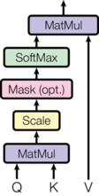
In practice, we compute the attention function on a set of queries simultaneously, packed together into a matrix $Q$. The keys and values are also packed together into matrices $K$ and $V$. We compute the matrix of outputs as:
\[\mathrm{Attention}(Q, K, V) = \mathrm{softmax}(\frac{QK^T}{\sqrt{d_k}})V\]def attention(query, key, value, mask=None, dropout=0.0):
"Compute 'Scaled Dot Product Attention'"
d_k = query.size(-1)
scores = torch.matmul(query, key.transpose(-2, -1)) \
/ math.sqrt(d_k)
if mask is not None:
scores = scores.masked_fill(mask == 0, -1e9)
p_attn = F.softmax(scores, dim = -1)
# (Dropout described below)
p_attn = F.dropout(p_attn, p=dropout)
return torch.matmul(p_attn, value), p_attnThe two most commonly used attention functions are additive attention (cite), and dot-product (multiplicative) attention. Dot-product attention is identical to our algorithm, except for the scaling factor of $\frac{1}{\sqrt{d_k}}$. Additive attention computes the compatibility function using a feed-forward network with a single hidden layer. While the two are similar in theoretical complexity, dot-product attention is much faster and more space-efficient in practice, since it can be implemented using highly optimized matrix multiplication code.
While for small values of $d_k$ the two mechanisms perform similarly, additive attention outperforms dot product attention without scaling for larger values of $d_k$ (cite). We suspect that for large values of $d_k$, the dot products grow large in magnitude, pushing the softmax function into regions where it has extremely small gradients (To illustrate why the dot products get large, assume that the components of $q$ and $k$ are independent random variables with mean $0$ and variance $1$. Then their dot product, $q \cdot k = \sum_{i=1}^{d_k} q_ik_i$, has mean $0$ and variance $d_k$.). To counteract this effect, we scale the dot products by $\frac{1}{\sqrt{d_k}}$.
Multi-Head Attention
Instead of performing a single attention function with $d_{\text{model}}$-dimensional keys, values and queries, we found it beneficial to linearly project the queries, keys and values $h$ times with different, learned linear projections to $d_k$, $d_k$ and $d_v$ dimensions, respectively. On each of these projected versions of queries, keys and values we then perform the attention function in parallel, yielding $d_v$-dimensional output values. These are concatenated and once again projected, resulting in the final values:
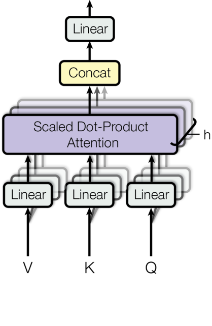
Multi-head attention allows the model to jointly attend to information from different representation subspaces at different positions. With a single attention head, averaging inhibits this. \(\mathrm{MultiHead}(Q, K, V) = \mathrm{Concat}(\mathrm{head_1}, ..., \mathrm{head_h})W^O \\ \text{where}~\mathrm{head_i} = \mathrm{Attention}(QW^Q_i, KW^K_i, VW^V_i)\)
Where the projections are parameter matrices $W^Q_i \in \mathbb{R}^{d_{\text{model}} \times d_k}$, $W^K_i \in \mathbb{R}^{d_{\text{model}} \times d_k}$, $W^V_i \in \mathbb{R}^{d_{\text{model}} \times d_v}$ and $W^O \in \mathbb{R}^{hd_v \times d_{\text{model}}}$. In this work we employ $h=8$ parallel attention layers, or heads. For each of these we use $d_k=d_v=d_{\text{model}}/h=64$. Due to the reduced dimension of each head, the total computational cost is similar to that of single-head attention with full dimensionality.
class MultiHeadedAttention(nn.Module):
    def __init__(self, h, d_model, dropout=0.1):
        "Take in model size and number of heads."
        super(MultiHeadedAttention, self).__init__()
        assert d_model % h == 0
        # We assume d_v always equals d_k
        self.d_k = d_model // h
        self.h = h
        self.p = dropout
        self.linears = clones(nn.Linear(d_model, d_model), 4)
        self.attn = None

    def forward(self, query, key, value, mask=None):
        "Implements Figure 2"
        if mask is not None:
            # Same mask applied to all h heads.
            mask = mask.unsqueeze(1)
        nbatches = query.size(0)

        # 1) Do all the linear projections in batch from d_model => h x d_k
        query, key, value = \
            [l(x).view(nbatches, -1, self.h, self.d_k).transpose(1, 2)
             for l, x in zip(self.linears, (query, key, value))]

        # 2) Apply attention on all the projected vectors in batch.
        x, self.attn = attention(query, key, value, mask=mask, dropout=self.p)

        # 3) "Concat" using a view and apply a final linear.
        x = x.transpose(1, 2).contiguous() \
             .view(nbatches, -1, self.h * self.d_k)
        return self.linears[-1](x)
Applications of Attention in our Model
The Transformer uses multi-head attention in three different ways: 1) In “encoder-decoder attention” layers, the queries come from the previous decoder layer, and the memory keys and values come from the output of the encoder. This allows every position in the decoder to attend over all positions in the input sequence. This mimics the typical encoder-decoder attention mechanisms in sequence-to-sequence models such as (cite).
2) The encoder contains self-attention layers. In a self-attention layer all of the keys, values and queries come from the same place, in this case, the output of the previous layer in the encoder. Each position in the encoder can attend to all positions in the previous layer of the encoder.
3) Similarly, self-attention layers in the decoder allow each position in the decoder to attend to all positions in the decoder up to and including that position. We need to prevent leftward information flow in the decoder to preserve the auto-regressive property. We implement this inside of scaled dot- product attention by masking out (setting to $-\infty$) all values in the input of the softmax which correspond to illegal connections.
Position-wise Feed-Forward Networks
In addition to attention sub-layers, each of the layers in our encoder and decoder contains a fully connected feed-forward network, which is applied to each position separately and identically. This consists of two linear transformations with a ReLU activation in between.
\[\mathrm{FFN}(x)=\max(0, xW_1 + b_1) W_2 + b_2\]While the linear transformations are the same across different positions, they use different parameters from layer to layer. Another way of describing this is as two convolutions with kernel size 1. The dimensionality of input and output is $d_{\text{model}}=512$, and the inner-layer has dimensionality $d_{ff}=2048$.
class PositionwiseFeedForward(nn.Module):
    "Implements FFN equation."
    def __init__(self, d_model, d_ff, dropout=0.1):
        super(PositionwiseFeedForward, self).__init__()
        # Torch linears have a `b` by default.
        self.w_1 = nn.Linear(d_model, d_ff)
        self.w_2 = nn.Linear(d_ff, d_model)
        self.dropout = nn.Dropout(dropout)

    def forward(self, x):
        return self.w_2(self.dropout(F.relu(self.w_1(x))))
Embeddings and Softmax
Similarly to other sequence transduction models, we use learned embeddings to convert the input tokens and output tokens to vectors of dimension $d_{\text{model}}$. We also use the usual learned linear transformation and softmax function to convert the decoder output to predicted next-token probabilities. In our model, we share the same weight matrix between the two embedding layers and the pre-softmax linear transformation, similar to (cite). In the embedding layers, we multiply those weights by $\sqrt{d_{\text{model}}}$.
class Embeddings(nn.Module):
    def __init__(self, d_model, vocab):
        super(Embeddings, self).__init__()
        self.lut = nn.Embedding(vocab, d_model)
        self.d_model = d_model

    def forward(self, x):
        return self.lut(x) * math.sqrt(self.d_model)
Positional Encoding
Since our model contains no recurrence and no convolution, in order for the model to make use of the order of the sequence, we must inject some information about the relative or absolute position of the tokens in the sequence. To this end, we add “positional encodings” to the input embeddings at the bottoms of the encoder and decoder stacks. The positional encodings have the same dimension $d_{\text{model}}$ as the embeddings, so that the two can be summed. There are many choices of positional encodings, learned and fixed (cite).
In this work, we use sine and cosine functions of different frequencies: \(PE_{(pos,2i)} = sin(pos / 10000^{2i/d_{\text{model}}})\)
\(PE_{(pos,2i+1)} = cos(pos / 10000^{2i/d_{\text{model}}})\) where $pos$ is the position and $i$ is the dimension. That is, each dimension of the positional encoding corresponds to a sinusoid. The wavelengths form a geometric progression from $2\pi$ to $10000 \cdot 2\pi$. We chose this function because we hypothesized it would allow the model to easily learn to attend by relative positions, since for any fixed offset $k$, $PE_{pos+k}$ can be represented as a linear function of $PE_{pos}$.
In addition, we apply dropout to the sums of the embeddings and the positional encodings in both the encoder and decoder stacks. For the base model, we use a rate of $P_{drop}=0.1$.
class PositionalEncoding(nn.Module):
    "Implement the PE function."
    def __init__(self, d_model, dropout, max_len=5000):
        super(PositionalEncoding, self).__init__()
        self.dropout = nn.Dropout(p=dropout)

        # Compute the positional encodings once in log space.
        pe = torch.zeros(max_len, d_model)
        position = torch.arange(0, max_len).unsqueeze(1)
        div_term = torch.exp(torch.arange(0, d_model, 2) *
                             -(math.log(10000.0) / d_model))
        pe[:, 0::2] = torch.sin(position * div_term)
        pe[:, 1::2] = torch.cos(position * div_term)
        pe = pe.unsqueeze(0)
        self.register_buffer('pe', pe)

    def forward(self, x):
        x = x + Variable(self.pe[:, :x.size(1)], requires_grad=False)
        return self.dropout(x)
# The positional encoding will add in a sine wave based on position.
# The frequency and offset of the wave is different for each dimension.
plt.figure(figsize=(15, 5))
pe = PositionalEncoding(20, 0)
y = pe.forward(Variable(torch.zeros(1, 100, 20)))
plt.plot(np.arange(100), y[0, :, 4:8].data.numpy())
plt.legend(["dim %d"%p for p in [4,5,6,7]])
None![]()
We also experimented with using learned positional embeddings (cite) instead, and found that the two versions produced nearly identical results. We chose the sinusoidal version because it may allow the model to extrapolate to sequence lengths longer than the ones encountered during training.
Generation
class Generator(nn.Module):
    "Standard generation step."
    def __init__(self, d_model, vocab):
        super(Generator, self).__init__()
        self.proj = nn.Linear(d_model, vocab)

    def forward(self, x):
        return F.log_softmax(self.proj(x), dim=-1)
Full Model
def make_model(src_vocab, tgt_vocab, N=6,
               d_model=512, d_ff=2048, h=8, dropout=0.1):
    "Helper: Construct a model from hyperparameters."
    c = copy.deepcopy
    attn = MultiHeadedAttention(h, d_model, dropout)
    ff = PositionwiseFeedForward(d_model, d_ff, dropout)
    position = PositionalEncoding(d_model, dropout)
    model = EncoderDecoder(
        Encoder(EncoderLayer(d_model, c(attn), c(ff), dropout), N),
        Decoder(DecoderLayer(d_model, c(attn), c(attn),
                             c(ff), dropout), N),
        nn.Sequential(Embeddings(d_model, src_vocab), c(position)),
        nn.Sequential(Embeddings(d_model, tgt_vocab), c(position)),
        Generator(d_model, tgt_vocab))

    # This was important from their code.
    # Initialize parameters with Glorot / fan_avg.
    for p in model.parameters():
        if p.dim() > 1:
            nn.init.xavier_uniform(p)
    return model
# Small example model.
tmp_model = make_model(10, 10, 2)Training
This section describes the training regime for our models.
Training Data and Batching
We trained on the standard WMT 2014 English-German dataset consisting of about 4.5 million sentence pairs. Sentences were encoded using byte-pair encoding \citep{DBLP:journals/corr/BritzGLL17}, which has a shared source-target vocabulary of about 37000 tokens. For English-French, we used the significantly larger WMT 2014 English-French dataset consisting of 36M sentences and split tokens into a 32000 word-piece vocabulary.
Sentence pairs were batched together by approximate sequence length. Each training batch contained a set of sentence pairs containing approximately 25000 source tokens and 25000 target tokens.
# Implemented in part below.Hardware and Schedule
We trained our models on one machine with 8 NVIDIA P100 GPUs. For our base models using the hyperparameters described throughout the paper, each training step took about 0.4 seconds. We trained the base models for a total of 100,000 steps or 12 hours. For our big models, step time was 1.0 seconds. The big models were trained for 300,000 steps (3.5 days).
# Our method is single GPU, although easy to extend.Optimizer
We used the Adam optimizer (cite) with $\beta_1=0.9$, $\beta_2=0.98$ and $\epsilon=10^{-9}$. We varied the learning rate over the course of training, according to the formula: \(lrate = d_{\text{model}}^{-0.5} \cdot \min({step\_num}^{-0.5}, {step\_num} \cdot {warmup\_steps}^{-1.5})\) This corresponds to increasing the learning rate linearly for the first $warmup_steps$ training steps, and decreasing it thereafter proportionally to the inverse square root of the step number. We used $warmup_steps=4000$.
# Note: This part is very important.
# Need to train with this setup of the model is very unstable.
class NoamOpt:
    "Optim wrapper that implements rate."
    def __init__(self, model_size, factor, warmup, optimizer):
        self.optimizer = optimizer
        self._step = 0
        self.warmup = warmup
        self.factor = factor
        self.model_size = model_size
        self._rate = 0

    def step(self):
        "Update parameters and rate"
        self._step += 1
        rate = self.rate()
        for p in self.optimizer.param_groups:
            p['lr'] = rate
        self._rate = rate
        self.optimizer.step()

    def rate(self, step = None):
        "Implement `lrate` above"
        if step is None:
            step = self._step
        return self.factor * \
            (self.model_size ** (-0.5) *
            min(step ** (-0.5), step * self.warmup**(-1.5)))

def get_std_opt(model):
    return NoamOpt(model.src_embed[0].d_model, 2, 4000,
    torch.optim.Adam(model.parameters(),
        lr=0, betas=(0.9, 0.98), eps=1e-9))
# Three settings of the lrate hyperparameters.
opts = [NoamOpt(512, 1, 4000, None),
NoamOpt(512, 1, 8000, None),
NoamOpt(256, 1, 4000, None)]
plt.plot(np.arange(1, 20000), [[opt.rate(i) for opt in opts] for i in range(1, 20000)])
plt.legend(["512:4000", "512:8000", "256:4000"])
None![]()
Regularization
Label Smoothing
During training, we employed label smoothing of value $\epsilon_{ls}=0.1$ (cite). This hurts perplexity, as the model learns to be more unsure, but improves accuracy and BLEU score.
class LabelSmoothing(nn.Module):
    "Implement label smoothing."
    def __init__(self, size, padding_idx, smoothing=0.0):
        super(LabelSmoothing, self).__init__()
        self.criterion = nn.KLDivLoss(size_average=False)
        self.padding_idx = padding_idx
        self.confidence = 1.0 - smoothing
        self.smoothing = smoothing
        self.size = size
        self.true_dist = None

    def forward(self, x, target):
        assert x.size(1) == self.size
        true_dist = x.data.clone()
        true_dist.fill_(self.smoothing / (self.size - 2))
        true_dist.scatter_(1, target.data.unsqueeze(1), self.confidence)
        true_dist[:, self.padding_idx] = 0
        mask = torch.nonzero(target.data == self.padding_idx)
        if mask.dim() > 0:
            true_dist.index_fill_(0, mask.squeeze(), 0.0)
        self.true_dist = true_dist
        return self.criterion(x, Variable(true_dist, requires_grad=False))
#Example of label smoothing.
crit = LabelSmoothing(5, 0, 0.1)
predict = torch.FloatTensor([[0, 0.2, 0.7, 0.1, 0],
[0, 0.2, 0.7, 0.1, 0],
[0, 0.2, 0.7, 0.1, 0]])
v = crit(Variable(predict.log()),
Variable(torch.LongTensor([2, 1, 0])))
# Show the target distributions expected by the system.
plt.imshow(crit.true_dist)
None![]()
# Label smoothing starts to penalize the model
# if it gets very confident about a given choice
def loss(x):
    d = x + 3 * 1
    predict = torch.FloatTensor([[0, x / d, 1 / d, 1 / d, 1 / d],
                                 ])
    #print(predict)
    return crit(Variable(predict.log()),
                 Variable(torch.LongTensor([1]))).data[0]
plt.plot(np.arange(1, 100), [loss(x) for x in range(1, 100)])
[<matplotlib.lines.Line2D at 0x2ba53d911550>]
![]()
In Practice
Computing the Loss Efficiently
def loss_backprop(generator, criterion, out, targets, normalize, bp=True):
    """
    Memory optmization. Compute each timestep separately and sum grads.
    """
    assert out.size(1) == targets.size(1)
    total = 0.0
    out_grad = []
    for i in range(out.size(1)):
        out_column = Variable(out[:, i].data, requires_grad=True)
        gen = generator(out_column)
        loss = criterion(gen, targets[:, i]) / normalize
        total += loss.data[0]
        loss.backward()
        out_grad.append(out_column.grad.data.clone())
    if bp:
        out_grad = torch.stack(out_grad, dim=1)
        out.backward(gradient=out_grad)
    return total
Training Setup
def make_std_mask(src, tgt, pad):
    "Create a mask to hide padding and future words."
    src_mask = (src != pad).unsqueeze(-2)
    tgt_mask = (tgt != pad).unsqueeze(-2)
    tgt_mask = tgt_mask & Variable(
        subsequent_mask(tgt.size(-1)).type_as(tgt_mask.data))
    return src_mask, tgt_mask

class Batch:
    "Batch object."
    def __init__(self, src, trg, src_mask, trg_mask, ntokens):
        self.src = src
        self.trg = trg
        self.src_mask = src_mask
        self.trg_mask = trg_mask
        self.ntokens = ntokens
def train_epoch(train_iter, model, criterion, opt):
"Standard Training and Logging Function"
model.train()
for i, batch in enumerate(train_iter):
src, trg, src_mask, trg_mask = \
batch.src, batch.trg, batch.src_mask, batch.trg_mask
out = model.forward(src, trg[:, :-1], src_mask, trg_mask[:, :-1, :-1])
loss = loss_backprop(model.generator, criterion,
out, trg[:, 1:], batch.ntokens)
model_opt.step()
model_opt.optimizer.zero_grad()
if i % 10 == 1:
print(i, loss, model_opt._rate)def valid_epoch(valid_iter, model, criterion):
"Standard validation function"
model.eval()
total = 0
total_tokens = 0
for batch in valid_iter:
src, trg, src_mask, trg_mask = \
batch.src, batch.trg, batch.src_mask, batch.trg_mask
out = model.forward(src, trg[:, :-1],
src_mask, trg_mask[:, :-1, :-1])
total += loss_backprop(model.generator, criterion, out, trg[:, 1:],
batch.ntokens, bp=False) * batch.ntokens
total_tokens += batch.ntokens
return total / total_tokensA Toy Example
def data_gen(V, batch, nbatches):
    "Generate random data for a src-tgt copy task."
    for i in range(nbatches):
        data = torch.from_numpy(np.random.randint(1, V, size=(batch, 10)))
        src = Variable(data, requires_grad=False)
        tgt = Variable(data, requires_grad=False)
        src_mask, tgt_mask = make_std_mask(src, tgt, 0)
        yield Batch(src, tgt, src_mask, tgt_mask, (tgt[1:] != 0).data.sum())
# Train the simple copy task.
V = 11
criterion = LabelSmoothing(size=V, padding_idx=0, smoothing=0.0)
model = make_model(V, V, N=2)
model_opt = get_std_opt(model)
for epoch in range(2):
train_epoch(data_gen(V, 30, 20), model, criterion, model_opt)
print(valid_epoch(data_gen(V, 30, 5), model, criterion))1 2.882607638835907 6.987712429686844e-07
11 2.5675880014896393 4.192627457812107e-06
2.3521071523427963
1 2.4410500079393387 7.686483672655528e-06
11 2.2494828701019287 1.118033988749895e-05
1.9590912282466888
A Real World Example
Finally we consider a real-world example using the IWSLT German-English Translation task. This task is much smaller than the WMT task considered in the paper, but it illustrates the whole system
# For data loading.
from torchtext import data, datasets
# Load words from IWSLT
#!pip install torchtext spacy
#!python -m spacy download en
#!python -m spacy download de
import spacy
spacy_de = spacy.load('de')
spacy_en = spacy.load('en')
def tokenize_de(text):
return [tok.text for tok in spacy_de.tokenizer(text)]
def tokenize_en(text):
return [tok.text for tok in spacy_en.tokenizer(text)]
BOS_WORD = '<s>'
EOS_WORD = '</s>'
BLANK_WORD = "<blank>"
SRC = data.Field(tokenize=tokenize_de, pad_token=BLANK_WORD)
TGT = data.Field(tokenize=tokenize_en, init_token = BOS_WORD,
eos_token = EOS_WORD, pad_token=BLANK_WORD)
MAX_LEN = 100
train, val, test = datasets.IWSLT.splits(exts=('.de', '.en'), fields=(SRC, TGT),
filter_pred=lambda x: len(vars(x)['src']) <= MAX_LEN and
len(vars(x)['trg']) <= MAX_LEN)
MIN_FREQ = 1
SRC.build_vocab(train.src, min_freq=MIN_FREQ)
TGT.build_vocab(train.trg, min_freq=MIN_FREQ)# Batching matters quite a bit.
# This is temporary code for dynamic batching based on number of tokens.
# This code should all go away once things get merged in this library.
BATCH_SIZE = 4096
global max_src_in_batch, max_tgt_in_batch
def batch_size_fn(new, count, sofar):
"Keep augmenting batch and calculate total number of tokens + padding."
global max_src_in_batch, max_tgt_in_batch
if count == 1:
max_src_in_batch = 0
max_tgt_in_batch = 0
max_src_in_batch = max(max_src_in_batch, len(new.src))
max_tgt_in_batch = max(max_tgt_in_batch, len(new.trg) + 2)
src_elements = count * max_src_in_batch
tgt_elements = count * max_tgt_in_batch
return max(src_elements, tgt_elements)
class MyIterator(data.Iterator):
def create_batches(self):
if self.train:
def pool(d, random_shuffler):
for p in data.batch(d, self.batch_size * 100):
p_batch = data.batch(
sorted(p, key=self.sort_key),
self.batch_size, self.batch_size_fn)
for b in random_shuffler(list(p_batch)):
yield b
self.batches = pool(self.data(), self.random_shuffler)
else:
self.batches = []
for b in data.batch(self.data(), self.batch_size,
self.batch_size_fn):
self.batches.append(sorted(b, key=self.sort_key))
def rebatch(pad_idx, batch):
"Fix order in torchtext to match ours"
src, trg = batch.src.transpose(0, 1), batch.trg.transpose(0, 1)
src_mask, trg_mask = make_std_mask(src, trg, pad_idx)
return Batch(src, trg, src_mask, trg_mask, (trg[1:] != pad_idx).data.sum())
train_iter = MyIterator(train, batch_size=BATCH_SIZE, device=0,
repeat=False, sort_key=lambda x: (len(x.src), len(x.trg)),
batch_size_fn=batch_size_fn, train=True)
valid_iter = MyIterator(val, batch_size=BATCH_SIZE, device=0,
repeat=False, sort_key=lambda x: (len(x.src), len(x.trg)),
batch_size_fn=batch_size_fn, train=False)# Create the model an load it onto our GPU.
pad_idx = TGT.vocab.stoi["<blank>"]
model = make_model(len(SRC.vocab), len(TGT.vocab), N=6)
model_opt = get_std_opt(model)
model.cuda()
Nonecriterion = LabelSmoothing(size=len(TGT.vocab), padding_idx=pad_idx, smoothing=0.1)
criterion.cuda()
for epoch in range(15):
train_epoch((rebatch(pad_idx, b) for b in train_iter), model, criterion, model_opt)
print(valid_epoch((rebatch(pad_idx, b) for b in valid_iter), model, criterion)) File "<ipython-input-383-b50fcff281d0>", line 3
break
^
SyntaxError: 'break' outside loop